4.1. Loading and visualizing data
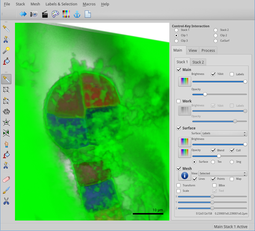
Figure 1: 16-cells embryo of Arabidopsis thaliana. Image: Saiko Yoshida, Weijer’s lab.
For this tutorial, download this dataset, which we used while working on [Yoshida2014].
4.1.1. Loading the data
There are four ways to load data in LithoGraphX.
- The simplest is to open the data directly with LithoGraphX. If you installed it correctly, data files native to LithoGraphX are associated with it. If you right-click on such a file you should have en entry to open it with LithoGraphX. Once launched, the data is simply loaded in the Stack 1, on the Main store for stacks.
- Once LithoGraphX is open, to load more data or replace existing data, the next simplest way is to use drag&drop. If you drop the file on the interaction area, it will be loaded in the currently active stack. For 3D images, you can also drop them on the main and store boxes in the main tab to load it at a particular location.
- You can use the menu to load either a LithoGraphX project, a stack or a mesh file. There are different menus for the various targets.
- You can directly use the loading processes: they are in the
Systemfolders of the Stack, Mesh and Global process tabs.
Try the various means to load the files 160112_4.tif, 160112_4.mgxm and
at last the project file 160112_4.lgxp.
4.1.2. Tuning the visualization
For this part, load only the TIFF file 160112_4.tif.
4.1.2.1. Opacity and basic transfer function
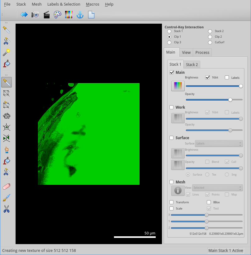
Figure 2: Initial view of the dataset.
When loading this dataset, you will see a very opaque object filling in almost the whole image. This is an embryo of Arabidopsis thaliana within its ovule, and we need to change the visual properties to start to see it.
But first, click the  button to see the transfer function (see
Figure 3).
button to see the transfer function (see
Figure 3).
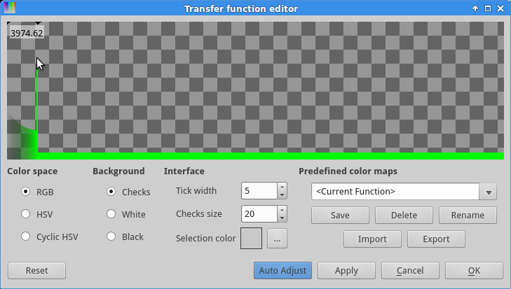
Figure 3: Transfer function of the object: note how only the low values are used.
We can see that the signal is entirely on the left of the spectrum! This is because the image is a 12 bits image. The number on the top-left indicate the value under the mouse cursor: a 12 bits image has a maximum possible value of 4095, while a 16 bits image can have values up to 65535. For further processing, we will want to expand the range of values. This will allow us to work with the representation with more ease, and will ensure fewer variations in the parameters of the data processing.
| Process | [Stack]Filters/Autoscale Stack |
|---|
The process Stack.Autoscale Stack in the Filters folder, will do just
that: rescale the stack to use the whole range of possible values. This process
has no parameter and will simply modify the current store. You will notice
a change in colour from green to cyan: this is because the result has been saved
in the work store of the stack 1, and this store is by default cyan. We can look
now at the transfer function of the work store (see Figure
4).
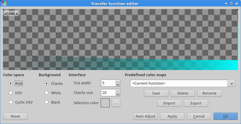
Figure 4: Scaled transfer function.
Now, we can see the stack uses the whole spectrum of values, which will be important later.
But to see the embryo, you need to decrease the opacity of the store (see Figure 5).

Figure 5: We need to adjust the opacity to reveal the embryo.
4.1.2.2. Surface and Mesh
Now, load the mesh, check the Blend check box and adjust the opacity.

Figure 6: Mesh covering the cells in the Embryo.
To look at the signal, we need first to create some. For example, compute the Gaussian curvature on each point:
| Process | [Stack]Signal/Project Mesh Curvature |
|---|---|
| Parameter | Value |
| Type | Gaussian |
| Neighborhood (μm) | 2 |
| Autoscale | Yes |
Then, click on the upper button to change the transfer
function of the signal (this is the second such button in the surface box). In
the dialogue box, select the “French flag” transfer function (see Figure
7).
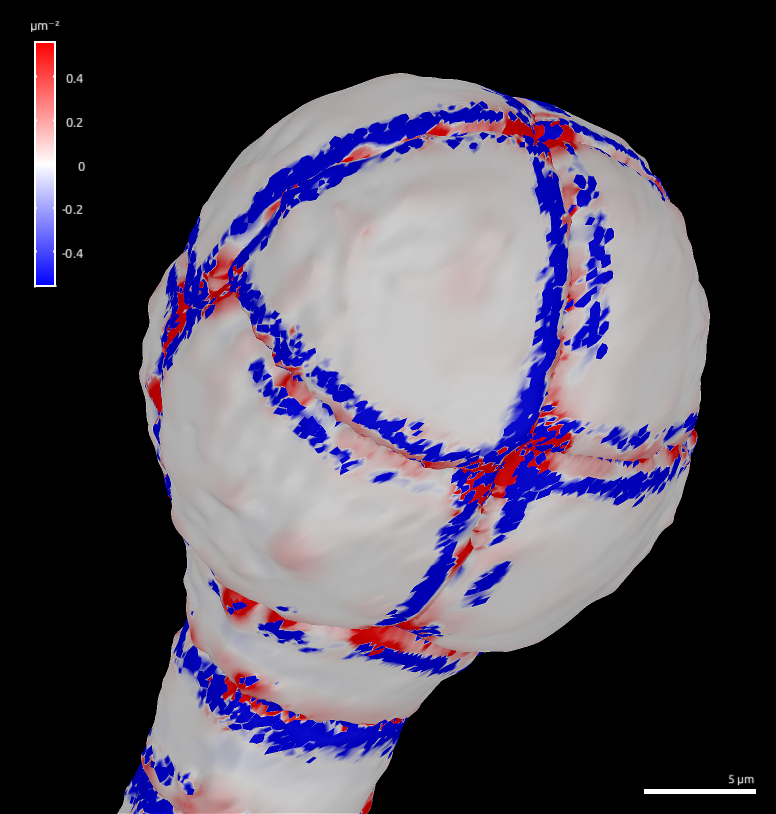
Figure 7: Curvature of the mesh.
Another property of the mesh is the heat. While the signal is per point, the heat is per label. THe main way to create a heat map is to use the process:
| Process | [Mesh]Heat Map/Heat Map |
|---|
When you launch the process, a fairly large dialogue box appear. Other tutorials will explain in more details what it is for. For now, simply change the heat map type fo “Volume” and make sure the visualization is “Geometry” (see Figure 8).
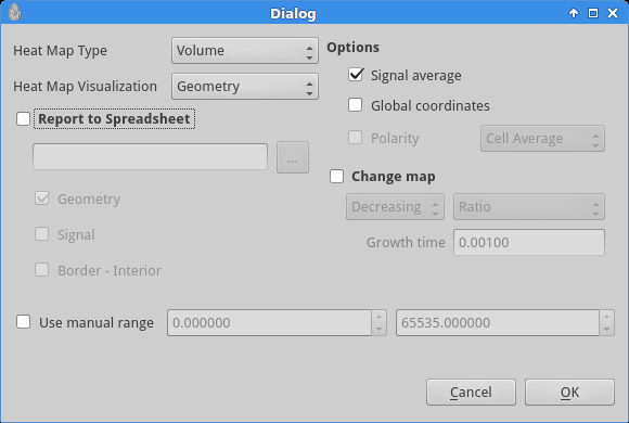
Figure 8: Dialog box of the Heatmap process.
After validation, the surface visualization automatically changed to “Heat” and displays the result (see Figure 9).
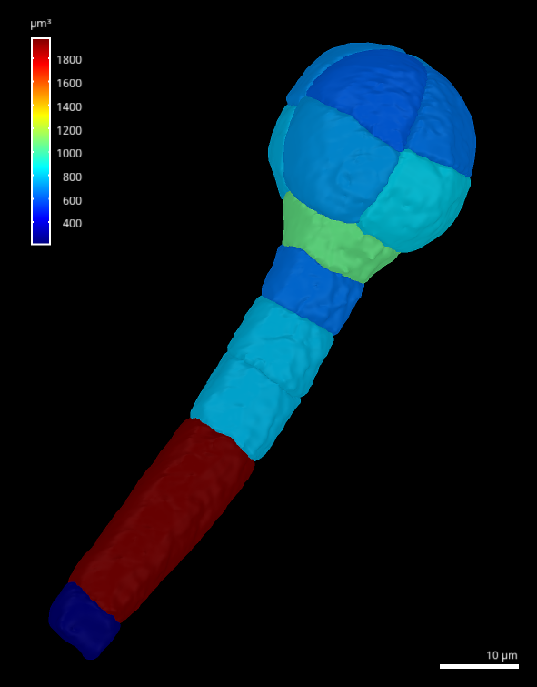
Figure 9: Head map of the cell volumes.
To change the transfer function, you can use the lower button.
4.1.2.3. Changing the colours
The main colours can be changed using the  button (see Figure
10).
button (see Figure
10).
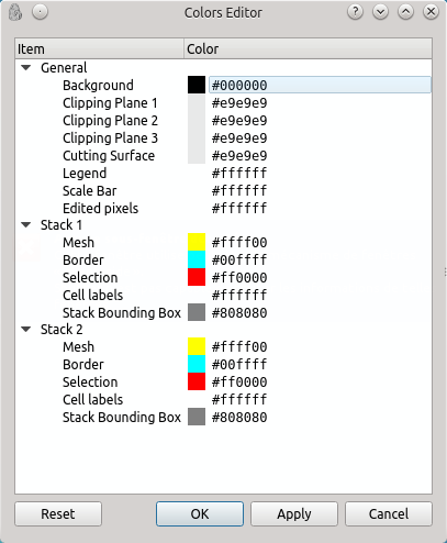
Figure 10: Colors Editor
For example, to re-create the image at the top of this page, change the background to white, and the legend and scale bar to black by double-clicking on the colour and use the dialogue box to choose the colour. To use if fully, you might also want to change the editing pixels and clipping planes colour to something darker.
4.1.2.4. Rendering speed
If rendering is slow, there are a number of settings in the View tab that can be helpful in the view quality box:
- Slices: changes the number of slices used to render the volume. The more the slower but also the better the quality. You can try to push it fully on the left to see how artefacts look like.
- Screen sampling: to speed up rendering while keeping a good image quality, LithoGraphX can reduce the image quality only when moving. This parameters sets the sub-sampling done while moving.
4.1.2.5. Transfer function
TODO
4.1.2.7. Processes
| [Yoshida2014] | Yoshida, S., Barbier de Reuille, P., Lane, B., Bassel, G. W., Prusinkiewicz, P., Smith, R. S. and Weijers, D. Genetic Control of Plant Development by Overriding a Geometric Division Rule Developmental Cell, 2014, 29, 75-87 |